Reference Station Classification
When using a network approach, expressing reliably GNSS position and velocities in a given reference frame (ITRF2014, IGS14, ETRF2000 or ETRF2014) requires the identification of ‘stable’ and ‘reliable’ reference stations. The choice of these reference stations can have a non-negligible impact on the estimated positions and velocities and of course on the derived geodynamic interpretations.
The EPN network has been set up to offer such reference stations: the reference positions and velocities of the EPN stations are kept up to date and are available through the EPN multi-year position and velocity solution. However, not all EPN stations are by definition suitable of reference stations.
To help the identification of the best EPN reference stations, a new station classification was developed. The criteria and thresholds used to define different classes for the EPN stations based on their performances are presented here.
In addition of the classification, we also developed a web tool to help the user to select the the most optimal EPN reference stations in a considered area and for a given observation time. The web tool is accessible here.
The Criteria
Time Series
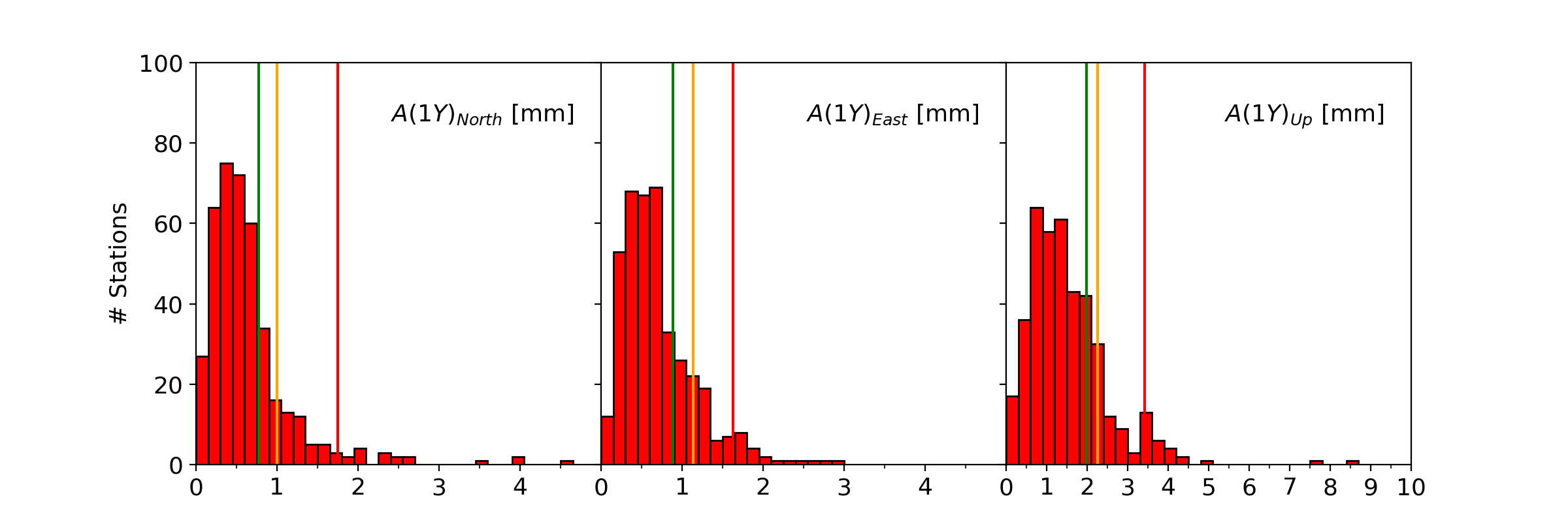
The residual position time series of the EPN stations are analyzed to quantify:
- the amplitude of the annual signal A(1Y)N, A(1Y)E, A(1Y)U on North, East and Up components
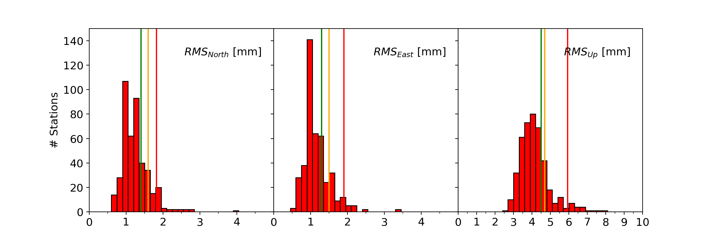
- the root mean square of the residual position time series after removing the annual and semi-annual signals RMSN, RMSE, RMSU on North, East and Up components
Reliability of the Velocity Estimation
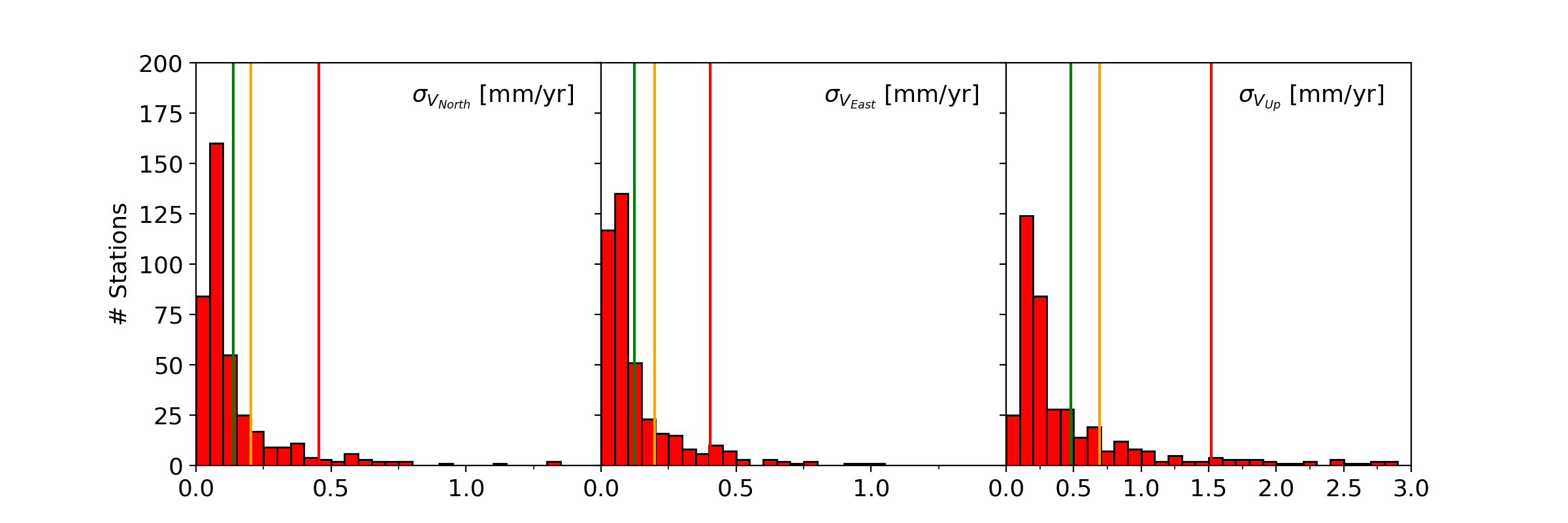
The EPN multi-year positions and velocities are estimated using CATREF software (Altamimi et al., 2007). CATREF is based on a least squares adjustment and neglects temporally correlated noise affecting the position time series. Therefore, the estimated velocity errors are too optimistic. In order to derive more realistic error estimates, the Hector software (Bos et al., 2013) has been used to estimate a linear trend, an annual and semi-annual signals assuming a temporal correlated noise (power-law + white noise). The Hector software (Bos et al., 2013) has been used to derive realistic error estimates. The comparison between Hector and CATREF velocity estimates is used to assess the reliability of the velocity estimation. The criteria used are:
- the realistic velocity error estimates from Hector (σVN, σVE,σVU) allow to assess the quality of the stations
- the differences between CATREF and Hector estimations (dVN, dVE, dVU) allow to assess the reliability of the velocity estimation

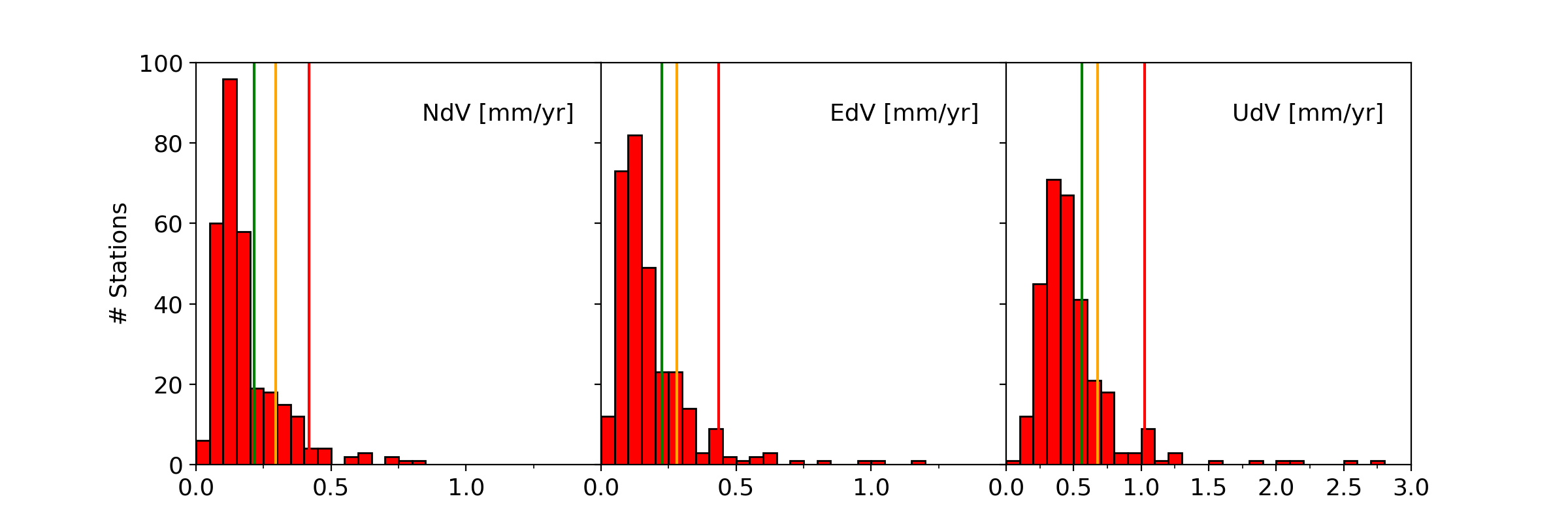
Velocity Variability
The variability over time of the estimated velocity for a station is obtained by comparing the velocities estimated using data from different moving time windows with the velocities obtained using the full data set of the station as it is included in the multi-year EPN solution.

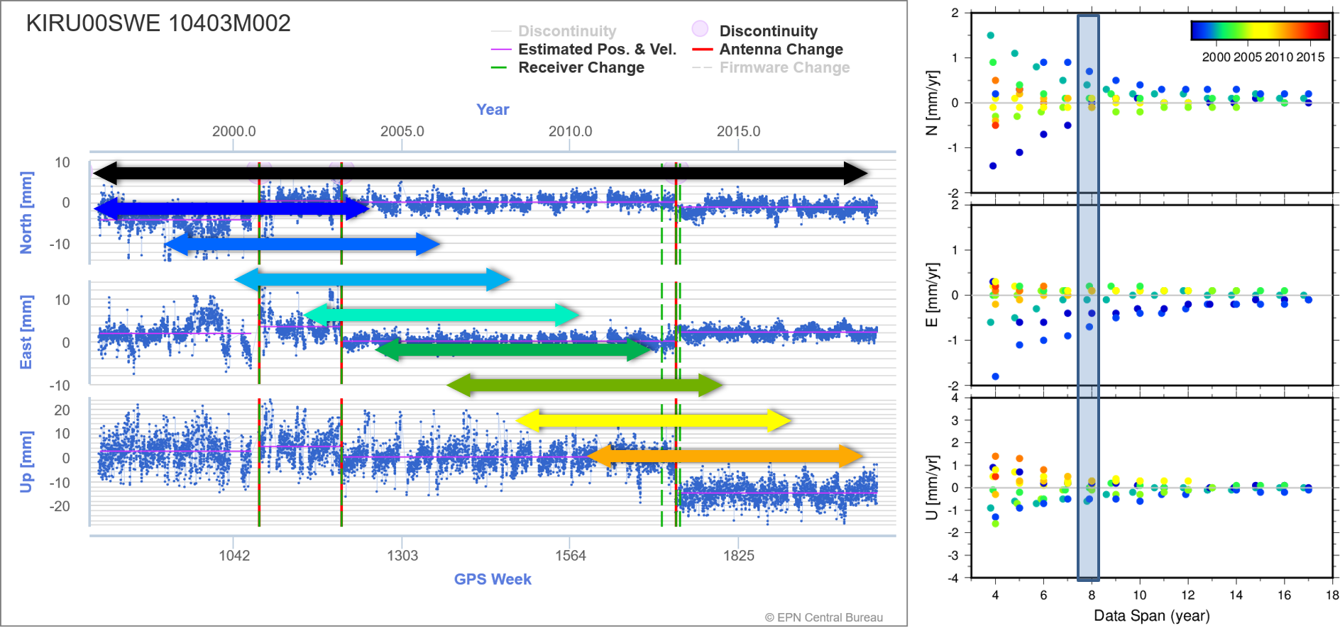
For each station and each component, the velocity variability NdV, EdV or UdV is then quantified as the RMS of the agreement between the station velocities obtained from the moving time windows (> 4 years) and the velocity obtained using the full time series.
The Thresholds and the Classification
Based on those criteria, the information has been organized and thresholds have been defined in order to end up with the station classification.
Thresholds
In order to find the stations having the best performances in the EPN network, the thresholds used are based on 3 different percentiles: percentile 75, 85 and 95. If the threshold is fixed at percentile 75, it means that the 25% worst stations for the considered criterion will be excluded. The idea behind this choice is that we want to reject the station that have the worst performances for each criterion.
Classification Rules
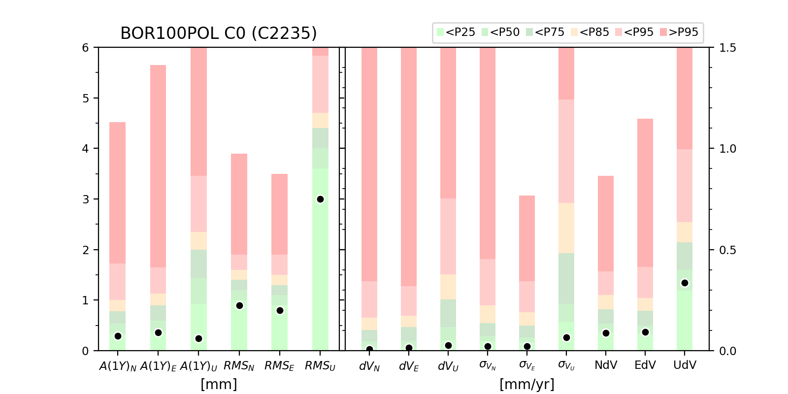
Class C0
This class contains the stations that behave better than the 75% best EPN stations and this on all the criteria.
It is the most stable and reliable stations in the EPN.
Class C1
The threshold on the velocity variability remains at percentile 75 as for C0, but the other criteria have been relaxed to the percentile 85 (excluding now the 15%, instead of 25%, worst EPN stations on the criteria for the reliability of the velocity estimation and the timeseries).
These stations are still very stable.
Class C2
The threshold on the velocity variability remains the same (percentile 75) as for C0 and C1. The threshold on the criteria for the reliability of the velocity estimation is the same as C1 (percentile 85). But, no thresholds have been applied for the criteria on the time series.
These stations are still stable, but they may be noisy or show some seasonal signals. Therefore, they may not be the best candidates as reference station for position solutions.
Class C3
The threshold on the velocity variability have been relaxed to percentile 85. The threshold on the criteria for the reliability of the velocity estimation or the time series are at percentile 85.
Compared to classes C0, C1, C2, those stations may be less stable in time and may present larger discrepancies when the time span is different from the EPN solution.
Class C4
The stations in this class do not have information on the velocity variability, because their time series are still too short, but the station perform better than percentile 85 on all the other criteria.
Those stations have a short history, but present satisfactory behaviour on all other criteria.
Class C5
The thresholds on the velocity variability remain at percentile 85. The threshold on the criteria for the reliability of the velocity estimation and the time series are relaxed to percentile 95.
These stations may not be suitable for some applications, the user has to check thoroughly the weak points of the station and its suitability for the user application.
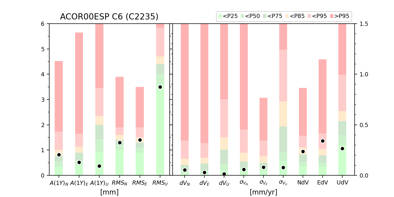
Class C6
The stations in this class perform badly in a least one of the criteria. 15% worst for the velocity variability and 5% worst for the other criteria such as the reliability of the velocity estimation or the time series .
These stations are not recommended as reference frame stations. If the user wants to use one of them, he has to understand the station weaknesses and thoroughly check if it fits his needs.
Class Short
Stations with less than 3 years of observations
No velocity is published for those stations.
Table2: the rules applied to define the 8 station classes C0, C1, C2, C3, C4, C5, C6, Short
| Name | Number | Criteria | Comment | ||||
|---|---|---|---|---|---|---|---|
| Velocity variability | Timeseries RMS | Amplitude 1Y signal | DVCatref-Hector | σHector | |||
| C0 | 64 | < Percentile 75 | < Percentile 75 | Most Stable Stations | |||
| C1 | 38 | < Percentile 75 | < Percentile 85 | ||||
| C2 | 47 | < Percentile 75 | No threshold | < Percentile 85 | Stable but Noisy or with Seasonal Signals | ||
| C3 | 19 | < Percentile 85 | < Percentile 85 | Less Stable | |||
| C4 | 11 | Not Available - Short time series | < Percentile 85 | ||||
| C5 | 72 | < Percentile 85 | No criteria > Percentile 95 | Even Less Stable | |||
| C6 | 146 | velocity variability > Percentile 85 and/or 1 or more other criteria > Percentile 95 or Short time series with 1 or more criteria > Percentile 85 | Less Reliable | ||||
| Short | 74 | < 3yr - not applicable | No velocity published | ||||